
I recently got hold of a copy of a very interesting book all about the development of the early PC game Wolfenstein 3D. Rather than being a history of ID Sofware, and the team that went on to develop the seminal games Doom and Quake (for which see here), it’s more of a review of the Wolfenstein 3D codebase (which is open source and available on GitHub) and a presentation of the challenges that were overcome in developing a groundbreaking 3D game for the PC with typical specs as of the time: i386, VGA graphics, Soundblaster sound card, running MS-DOS with perhaps 2MB RAM.
A PC of that era had significantly more CPU horsepower (in terms of MIPS) than any of the contemporary games consoles and that was what made it appealing as a target platform for a 3D game. The nature of the segmented memory model that DOS imposed (as a consequence of being tied to Real Mode on the 386), the architecture of the VGA graphics card and the lack of hardware floating point on the 386 presented lots of challenges to the project, and the strategies that Carmack and co. came up with to make it all work are ingenius and very interesting. It’s a good read … for those of a more geeky persuasion anyway. People like me, and - I suppose - you too dear reader.
All this is very interesting but not really the subject of this blog post. This post is a follow up to a previous one I wrote about the floating point representation of real numbers and was inspired by a description of floating point from this book that was unlike any that I have seen before. It represented a different way to think about that particular numeric format and, I think, is a very helpful way to try to visualize (and understand) how it was designed. I also realized that I’d left out descriptions of the “special” floating point values in my previous article and I needed to remedy that. So here we go. Onward!
The Traditional View
The traditional description of floating point representation involves the presentation of the following pattern of the 32 bits in a regular float in memory …
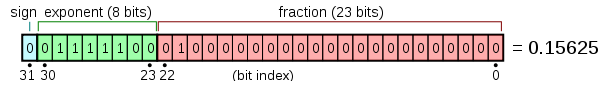
… and the following expression involving a sum of powers of 2 …
\[value = (-1)^{s} \times (1 + m) \times 2^e\]where \( s = b_{31} \), \( e = e_{biased} - 127 \), \( e_{biased} = \sum_{i=23}^{30}{b_i2^{i-23}} \) and \(m = \sum_{i=22}^{0}{b_i}2^{i-23}\).
It then proceeds to inform you that one bit of memory is used to indicate the sign of the number (the value \(s\) in the expression, where 0 indicates positive and 1 indicates negative), eight are used to represent the biased exponent (the value \(e_{biased}\)) and 23 are used to store the digits of what is known as the mantissa where there is an assumed leading 1 bit and the stored bits are assumed to be the part to the right of the binary point (the equivalent of the decimal point in the decimal representation of a real number). These are bits \(b_i\) for \(i\) in \([22, 0]\).
The Alternative View
An alternative spin on things is to observe that the floating-point representation of a number is an approximation to a given real number \(R\) as follows …
- First we note whether \(R\) is positive or negative and save that in a value (which we will call \(s\)) where positive will be stored as \(0\) and negative will be stored as \(1\)
- Then we determine which two consecutive powers of \(2\) bound \(|R|\) (the absolute value of \(R\)) above and below. Let’s denote these two values as \(2^e\) and \(2^{e+1}\).
- Next we divide the difference between \(2^e\) and \(2^{e+1}\) into \(N\) equal parts and find the number \(n\) such that \(2^e + \frac{n}{N} <= |R| < 2^e + \frac{n + 1}{N}\)
- The floating point approximation to \(R\) is parameterized by the values \(s\), \(e\), \(N\) and \(n\)
So we basically map out a comb of \(N\) discrete values between each two consecutive powers of \(2\) (within a range of such powers, \(2^{e_{min}}\) and \(2^{e_{max}}\)) and approximate \(|R|\) as the closest tooth of the comb equal to or less than \(|R|\).
I hope you can see that the accuracy of this approximation will depend on \(N\). The larger the value, the finer grain the divisions between the bounding powers of two will be and the closer we can get to the actual value of \(|R|\). I also hope you can see that the range of possible values we can approximate (from smallest to largest) will depend on \(e_{min}\) and \(e_{max}\).
Examples
Let’s look at some examples to illustrate things. We’ll assume that \(N\) is 8 for now and look at how we would represent the real numbers \(0.05\), \(6\) and \(50\).
First, \(0.05\). This number falls between \(2^{-5} = \frac{1}{32} = 0.03125\) and \(2^{-4} = \frac{1}{16} = 0.0625\) and the gap between the teeth of our comb will be \(\frac{2^{-5}}{8} = \frac{1}{256} = 0.00390625\).
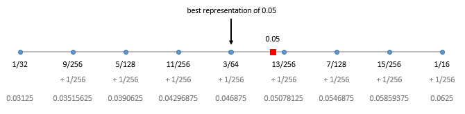
We can see that we can’t represent \(0.05\) perfectly and end up using \(\frac{3}{64} = 0.046875\) as an approximation.
Next, 6. This number falls between \(2^2 = 4\) and \(2^3 = 8\) and the gap between the teeth of our comb will be \(\frac{2^2}{8} = \frac{1}{2} = 0.5\).
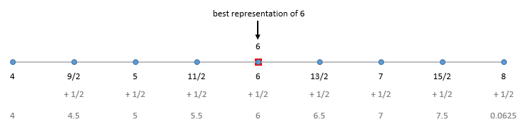
In this case we can represent \(6\) perfectly and so we do.
Finally, 50. This number falls between \(2^5 = 32\) and \(2^6 = 64\) and the gap between the teeth of our comb will be \(\frac{2^5}{8} = 4\).
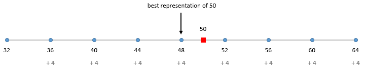
Again, we can’t represent \(50\) perfectly. The best we can do, within the bounds of the parameters we have chosen, is to use \(48\) as an approximation.
Mapping Between the Two Views
How does this view map to the traditional view of floating point and to the bit representation that we saw before?
Well, the sign flag \(s\) should be obvious; it maps to the sign bit.
The value \(N\) from the new view is equal to the maximum value that can be stored in the mantissa bits of the bit representation. In a regular 32 bit float there are 23 bits to store the mantissa. The maximum (unsigned) integer value that you can store in 23 bits is \(2^{23} = 8{,}388{,}608 \) and so, in a 32 bit float, the range between consecutive powers of two is quantized into \(8{,}388{,}608\) parts.
Finally we need to think about the range of possible values for the first power in the pair of consecutive powers of \(2\). We referred to this before as \([2^{e_{min}}\), \(2^{e_{max}}]\). In a 32 bit float, 8 bits are used to store a biased exponent which can take any value from the range \([0, 255]\). This is a biased exponent and the actual exponent (in the sum interpretation of float) is equal to \(\texttt{stored_exponent} - 127\). Thus the actual exponent can take any value in the range \([-127, 128]\). Therefore our pair of consecutive powers of \(2\) can be anything from \([2^{-127}, 2^{-126}]\) to \([2^{128}, 2^{129}]\).
Remember the traditional view …
where \(e = e_{biased} - 127\), \(e_{biased} = \sum_{i=23}^{30}{b_i2^{i-23}}\) and \(m = \sum_{i=22}^{0}{b_i}2^{i-23}\)
Here’s the alternate view …
\[value = (-1)^{s} \times (2^e + \frac{n}{N})\]where \(n = \sum_{i=0}^{22}{b_i2^i}\) and \(N = 2^{23}\)
Some Observations
The choice of \(N\) is critical and represents the granularity of the quantization that we impose on the ranges between consecutive powers of \(2\). The quantum is equal to \(\frac{1}{N}\).
The mantissa \(m\) represents how many quanta we add to the first power of \(2\).
The choice of storage size for \(e\) is critical and dictates the extremities of the range of values that we can represent.
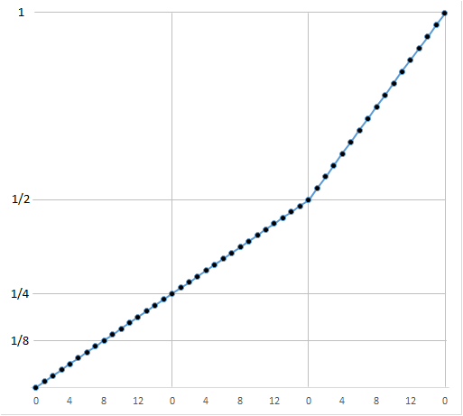
We always use the same granularity of quantization (the same number of bins) regardless of the power of \(2\) at the start of the range. This means that the absolute size of each bin (our quantum of value) grows the larger the number that we are representing. It also means that the relative size of each bin, relative to the starting value of the range remains the same for all ranges though. We can see this in the following image …
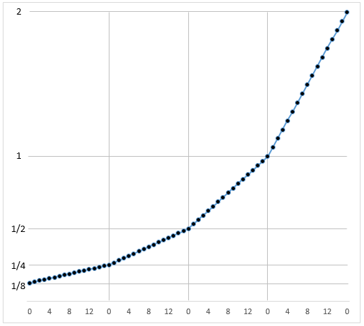
Here we are breaking each range into \(16\) bins. Each range is progressively wider but the number of bins remains the same. Each bin between \(1\) and \(2\) is wider than each bin between \(\frac{1}{8}\) and \(\frac{1}{4}\).
Special Values
Floating point uses a few special values. These are \(0\), \(\texttt{Infinity}\), \(\texttt{NaN}\) (short for Not a Number) and Denormalized Numbers; and there are actually two kinds of \(\texttt{NaN}\) value: Signalling and Quiet. More on the difference between Signalling and Quiet in a moment. For now let’s look at the representation of these values.
\(0\) is indicated by \(e_{biased} = 0\) and \(m = 0\). This leaves two possibilities for the sign bit and so there are actually two values \(+0\) and \(-0\).
\(\texttt{Infinity}\) is indicated by \(e_{biased} = 255\) and \(m = 0\). Again the sign can be \(0\) or \(1\) and so there are actually two values \(+\texttt{Infinity}\) and \(-\texttt{Infinity}\).
There are lots of \(\texttt{NaN}\) values. Any value with \(e_{biased} = 255\) and \(m != 0\) is considered \(\texttt{NaN}\). Signalling \(\texttt{NaN}\) values have the most significant bit of \(m\) (i.e. \(b_{22}\)) set to \(0\) and Quiet \(\texttt{NaN}\) values have it set to \(1\).
Signalling vs. Quiet …
Various floating point operations can generate an invalid result (i.e. dividing by zero) and such operations will return a value of \(\texttt{NaN}\). Whether the operation results in a Signalling \(\texttt{NaN}\) or a Quiet \(\texttt{NaN}\) gets into the arcana of floating point unit (FPU) implementation and is beyond my current knowledge. I can say though that if an operation results in a Quiet \(\texttt{NaN}\) then there is no indication that anything is unusual until the program checks the result and sees the \(\texttt{NaN}\). That is, computation continues without any signal from the FPU (or library if floating-point is implemented in software). However a Signalling \(\texttt{NaN}\) will immediately produce a signal, usually in the form of exception from the FPU. Whether the exception is thrown depends on the state of the FPU.
Denormalized Numbers …
These are represented by \(e_{biased} = 0\). This state indicates a slightly different interpretation of the rest of the bits in the value. Denormalized numbers are a special case used to smooth out the progression of represented numbers into and through \(0\). When \(e_{biased} = 0\) we use this formula for the value …
\[value = (-1)^{s} \times (m) \times 2^{e + 1}\]… as opposed to the regular …
\[value = (-1)^{s} \times (1 + m) \times 2^e\]Or with our alternate view …
\[value = (-1)^{s} \times (\frac{n}{N})\]… as opposed to …
\[value = (-1)^{s} \times (2^e + \frac{n}{N})\]One Final Picture or two, or three …
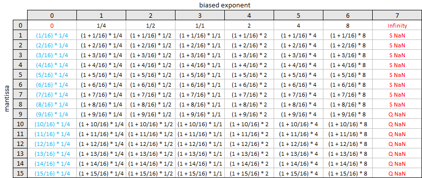
To close let’s imagine a hypothetical one byte floating point format with 1 bit for the sign, 3 bits for the biased exponent and 4 bits for the mantissa. In this format, \(e_{biased}\) can range from \(0\) to \(7\) and \(m\) can range from \(0\) to \(15\). We can show all the possible values in a grid, as the rational values …
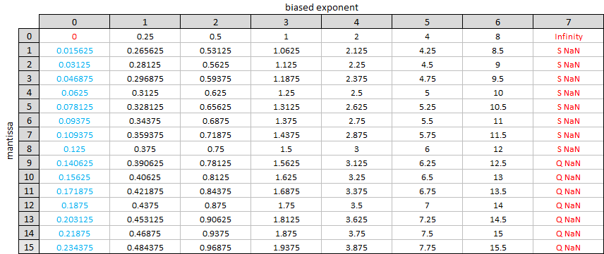
… and as the corresponding decimal values …
The values above include the denormalized numbers. To see the smoothing effect that these have let’s look at a picture showing the values of our representation near \(0\) with and without denormalization. First without …
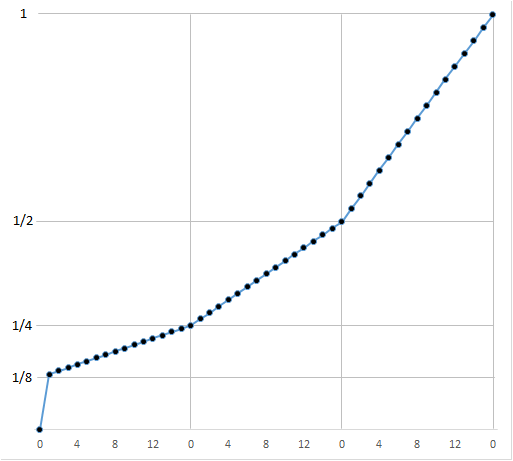
… and now with …
Much smoother.
Other Resources
Lots of people have written about floating point online. I have no illusions that my witterings are especially insightful or worthy. I have cribbed much of my knowledge from other places on the web actually. Here are some links to such resources. Go read more on the subject.